1. Provide a detailed explanation of why the Halting problem is considered unsolvable and its implications in Computer Science.

The Halting Problem is a famous problem in computer science. It was first explained by Alan Turing in 1936.

“Can we write a program that can check whether any other program will stop (halt) or run forever on a given input?”

Let’s suppose we have a program called Checker that can solve the Halting Problem. It takes two inputs:

• A program P
• An input I for that program

It gives:

• “Yes” if P stops when given I
• “No” if P runs forever on I

Now, we make a new program called TrickProgram, which uses Checker in a tricky way:

• If Checker says P halts → TrickProgram runs forever
• If Checker says P runs forever → TrickProgram stops

Now, give TrickProgram itself as input. This leads to a contradiction:

• If it says it halts → it runs forever
• If it says it runs forever → it halts

This is a logical contradiction, which means our assumption is wrong. So, such a Checker program cannot exist.

Therefore, the Halting Problem is unsolvable — no program can decide for all other programs whether they will halt or not.

The Halting Problem shows that there are limits to what computers can do. It means we cannot always write programs that check if other programs will stop or run forever. This affects how we build software tools, because no tool can perfectly detect all errors or infinite loops. It also teaches us that some problems in computer science cannot be solved by any program at all.

1. Limits of Computation:
   • It proves that not all problems can be solved using computers.
   • Some problems will never have a general algorithm to solve them.
2. No Perfect Program Checker:
   • We cannot create a program that can perfectly check if other programs will work correctly in all cases.
   • For example, we can’t always know if a program has infinite loops.
3. Impact on Software Tools:
   • Tools like compilers, debuggers, and antivirus software cannot always detect all errors or harmful behavior.
   • They may miss problems or give false alarms because of the Halting Problem.
4. Incomputable Problems Exist:
   • Some problems are undecidable (unsolvable by any program), just like the Halting Problem.
   • These problems need special approaches or may not be solvable at all.
5. Encourages Careful Programming:
   • Since we can’t always predict program behavior, programmers need to be careful with loops, conditions, and testing.

2. Discuss the characteristics of search problems and compare the efficiency of Linear search and Binary search algorithm.

Search algorithms are designed to find specific elements or a set of elements within a dataset. They are critical for tasks such as information retrieval, database queries, and decision-making processes. Search problems involve finding a specific item or solution from a large set of possibilities. The following are key characteristics:

1. Initial State: The starting point of the search (e.g., start of the list).
2. Goal State: The condition that defines when the solution is found (e.g., item matches the target).
3. State Space: The total set of possible states or configurations the search algorithm explores.
4. Operators/Actions: Rules or steps that move from one state to another (e.g., move to the next element).
5. Path to Goal: The sequence of steps taken to reach the solution.
6. Cost Function (Optional): Measures the effort (like time or steps) to reach a goal state.
7. Search Strategy: The method used to decide which paths to explore (e.g., linear vs. binary).
8. Performance Evaluation: Based on: Time Complexity, Space Complexity, Completeness, Optimality.

A linear search is a straightforward method for finding an item in a list. You check each item one by one until you find what you’re looking for. Here’s how it works,

Start at the Beginning: Look at the first item in the list.

Check Each Item: Compare the item you are looking for with the current item.

Move to the Next: If they don’t match, move to the next item in the list.

Repeat: Continue this process until you find the item or reach the end of the list.

Example: Suppose you have a list of city names: [Karachi, Lahore, Islamabad, Faisalabad]

And you want to find out if Islamabad is in the list.

Start with Karachi. Since Karachi isn’t Islamabad, move to the next city.

Next is Lahore. Lahore is not Islamabad, so move to the next city.

Now you have Islamabad. This is the city you’re looking for!

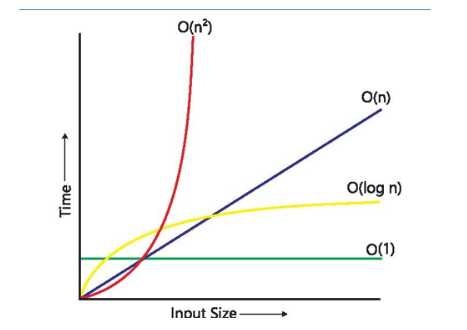
In this case, you’ve found Islamabad in the list. If Islamabad weren’t in the list, you would check all the cities one by one and then conclude that it’s not there. This method is called a linear search because you check each item in a straight line, from start to finish. Time complexity of linear search is O(n).

Binary Search is an efficient algorithm for finding an item in a sorted list. It works by repeatedly dividing the search interval in half and discarding the half where the item cannot be, until the item is found or the interval is empty.

Complexity:
The time complexity of binary search is O(log n) making it much faster than linear search algorithm, especially for large datasets.

3. Discuss the nature of optimization problems and provide examples of their applications in real-world scenarios.

An optimization problem is a type of problem in which we try to find the best solution from many possible options.

The word “optimize” means to make something as good as possible for example, saving time, getting higher marks, using less money, or gaining more profit.

The goal is to either:

• Minimize something (like time, cost, distance), or
• Maximize something (like profit, speed, marks).

Optimization problems are found in almost every field where decisions need to be made smartly under some limitations.

By solving optimization problems, we can save time, reduce cost, increase productivity, and make better decisions in real-world situations.

Objective Function (Target):
What we want to maximize or minimize
e.g., Maximize marks, minimize cost

Decision Variables (Choices):
The things we can change or decide
e.g., How many hours to study each subject

Constraints (Rules or Limits):
The restrictions or conditions we must follow
e.g., Only 5 hours available in a day

Example Area	How Optimization is Used
Study Timetable	Choosing the best schedule to study all subjects in limited time.
Exams Preparation	Maximizing marks by focusing more on important chapters.
Travel/Transport	Finding the shortest or fastest route to reach college.
Pocket Money Usage	Spending money wisely to get maximum benefit within your budget.
Classroom Management	Arranging students or seats for best discipline and attention.
Computer Programs	Making the code run faster by using less memory and time.

4. Explain the process and time complexity of the Bubble Sort algorithm. Compare it with another sorting algorithm of your choice in terms of efficiency.

Sorting algorithms are used to arrange data in a particular order, such as ascending or descending. Sorting is a fundamental operation that often serves as a prerequisite for other tasks like searching and data analysis.

Bubble Sort is one of the simplest sorting algorithms. It works by repeatedly stepping through the list, comparing adjacent elements, and swapping them if they are in the wrong order. This process is repeated until the list is sorted.

Process:

• Start from the beginning of the list.
• Compare each pair of adjacent elements.
• Swap them if they are in the wrong order.
• Continue the process until no more swaps are needed.

Example:
Consider the list [5, 3, 8, 4, 2]. Bubble Sort will first compare 5 and 3, swap them, then move to the next pair (5 and 8), and so on. After several passes through the list, the algorithm will sort the list as [2, 3, 4, 5, 8].

Complexity:
The time complexity of Bubble Sort is O(n²), making it inefficient for large datasets. However, it is easy to understand and implement, making it useful for educational purposes and small datasets.

Selection Sort is another simple sorting algorithm. It works by selecting the smallest (or largest, depending on the desired order) element from the unsorted part of the list and swapping it with the first element of the unsorted part. This process is repeated for the remaining unsorted portion of the list.

Process:

• Find the minimum element in the unsorted part of the list.
• Swap it with the first unsorted element.
• Move the boundary of the sorted and unsorted sections by one element.
• Repeat the process for the remaining elements.

Example:
For the list [29,10,14,37,13], Selection Sort will first find the smallest element, 10, and swap it with 29. The list becomes [10,29,14,37,13]. The process continues until the list is fully sorted.

Complexity:
The time complexity of Selection Sort is O(n²). Like Bubble Sort, it is not efficient for large datasets but is straightforward to implement.

5. Discuss the differences between time complexity and space complexity. How do they impact the choices of an algorithm for a specific problem?

Time complexity is a measure of how the running time of an algorithm increases as the size of the input data grows. It helps us understand how efficiently an algorithm performs when dealing with larger amounts of data.

Example: Consider the task of sorting a list of numbers. If the list contains only a few numbers, the task might be quick. However, as the volume of numbers increases, the time required to sort them also increases. Time complexity allows us to predict how this runtime scales with the input size.

Space complexity measures how the amount of memory or space an algorithm uses changes as the size of the input data increases. It helps us understand how efficiently an algorithm uses memory when handling large datasets.

Example: If an algorithm needs to store a list of numbers, its space complexity tells us how much memory will be required as the volume of numbers increases.

Feature	Time Complexity	Space Complexity
What it measures	How long an algorithm takes to run	How much memory an algorithm uses during execution
Unit of measure	Steps or operations (relative to input size n)	Bytes, kilobytes, or just memory units (also relative to n)
Focus	Speed: “How fast can you finish this?”	Storage: “How much space do you need to do it?”
Why it matters	Affects how quickly results are produced	Affects whether the algorithm can even run on the system
Example	Bubble Sort: O(n²) — terribly slow	Storing all possible results in memory: O(n²) — memory hog

1. Feasibility: Time and space complexity help determine if an algorithm can even handle the expected input size.
2. Classification: Different algorithm types (e.g., greedy, dynamic programming, divide & conquer) have distinct complexity patterns that guide their use.
3. Scalability: Efficient algorithms (e.g., O(n log n)) are necessary for large inputs, while simpler ones may suffice for small data.
4. Trade-offs: Sometimes we trade time for space (faster but memory-heavy) or vice versa (slower but memory-efficient).
5. Comparison: Complexity analysis allows objective comparison between multiple algorithms solving the same problem.